Markets Week Ahead: Gold Dips as Stocks Fly; EUR/USD, GBP/USD Await US Inflation

Markets Week Ahead: Gold Dips as Stocks Fly; EUR/USD, GBP/USD Await US Inflation

In the FX market, the U.S. dollar climbed for the fourth consecutive week, although gains were limited. In this context, both EUR/USD and GBP/USD edged lower, but ultimately managed to hold above key support levels. USD/JPY, meanwhile, rallied strongly, coming close to regaining the 150.00 handle.

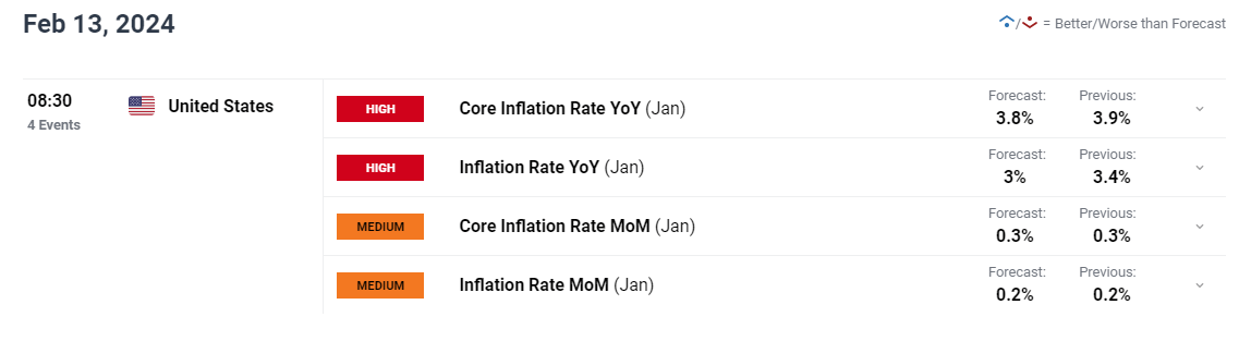
Looking ahead, volatility could accelerate in the new week, courtesy of a high-impact event on the U.S. economic calendar: the release of January inflation data on Tuesday. This could mean treacherous market conditions, so traders should be prepared for the possibility of wild price swings across assets.

UPCOMING US CPI REPORT

image2.png

Gain access to an extensive analysis of gold’s fundamental and technical outlook in our complimentary Q1 trading forecast. Download the guide now for valuable insights!

In the grand scheme of things, a hotter-than-expected U.S. CPI report should be positive for U.S. yields and the U.S. dollar, but bearish for stocks and gold prices. The S&P 500 and Nasdaq 100, for instance, may face challenges in sustaining their upward trajectory if progress on disinflation disappoints.

On the flip side, if inflation numbers surprise to the downside, the opposite scenario is likely to unfold, resulting in lower yields and a weaker U.S. dollar. This, in turn, should provide support for both equities and precious metals, at least in the short term.

For a comprehensive analysis of the factors that may influence financial markets and become a potential source of volatility in the upcoming trading sessions, check out the following selection of key forecasts compiled and prepared by the DailyFX team.

Seeking actionable trading ideas? Download our comprehensive trading opportunities guide, filled with insightful strategies tailored for the first quarter!

 FUNDAMENTAL AND TECHNICAL FORECASTS

British Pound Weekly Forecast: Busier Data Week Might Be Bruising

Sterling remains relatively elevated despite recent US Dollar strength. This week may make life a bit tougher for Sterling bulls.

Gold Price Forecast: US Inflation to Dictate Direction, Volatility Looms Ahead

This article discusses the fundamental and technical outlook for gold prices ahead of next week’s key U.S. inflation data, examining possible scenarios that could develop in the near term.

US Dollar Forecast: EUR/USD, GBP/USD and USD/JPY Price Action Setups

Next week US CPI headlines the schedule of high importance data. This forecast considers how major currency pairs shape up ahead of the US CPI release.

Understanding Inflation and its Global Impact

Understanding Inflation and its Global Impact

What is Inflation?

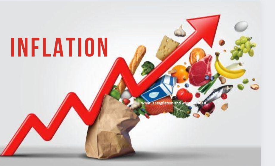
Inflation is the rise in prices of goods and services in an economy over a period of time, and is often displayed in percentage form. For example, if inflation is 2%, this suggests that prices are (on average) 2% higher than the previous period. Therefore, if a bottle of water cost $1 last year then this year it should be around $1.02. Inflation can result in significant costs to an economy as the purchasing power of individuals fall.

Deflation

Deflation is the opposite of inflation where prices fall. This suggests low demand for goods and services and often leads low interest rates. Deflation is atypical amongst developed countries.

Stagflation vs Hyperinflation

Stagflation occurs when an economy is stagnant (low growth) but inflation is still prevalent. This can occur when external factors impact an economy such as the price of oil.

Hyperinflation is an extremely high rate of inflation within an economy. Hyperinflation can be caused by an increase in money supply which consequently results in increased consumer spending and higher demand for goods and services.

Both deflation and hyperinflation can be detrimental to an economy and can result in higher rates of unemployment and lower growth. This makes the role of central banks critically important to control inflation as a lack of stability may have the potential for destructive penalties.

Measuring Inflation

Consumer Price Index (CPI)

This is one of the more common ways of measuring inflation, calculating inflation is based on a basket of goods and services which are often referred to as a ‘cost-of-living index’. Common cost-of-living indexes are the Consumer Price Index (CPI) and Retail Price Index (RPI). These measures relate to inflation experienced by consumers on a daily basis. Each central bank faces unique headwinds in selecting appropriate items to include within their inflation calculation.

Core CPI vs Headline CPI:

Two common phrases when dealing with inflation is ‘core’ and ‘headline’ CPI. This differentiating factor between the two terms is quite simple. Core CPI refers to the omission of food and energy prices from the Consumer Price Index while headline CPI includes both food and energy prices.

Producer Price Index (PPI)

The Producer Price Index (PPI) focuses on inflation at the early stages of production which can provide essential information for manufacturers and industry. The chart below shows the historical comparison between the different inflation measures (CPI, PPI and GDP Deflator). It is clear that PPI is the most volatile which can be explained in part by producers being unable to pass on relatable costs to the consumer in difficult periods such as the global financial crisis.

GDP Deflator

Another way to measure inflation is via the GDP deflator which takes into account domestic goods only while CPI and/or RPI includes foreign goods, as well. A second key difference is that the GDP deflator method encompasses all goods and services while CPI and/or RPI only measures the price of goods and services bought by consumers. Because the GDP deflator is not restricted by a fixed basket of goods, it has an advantage over the others.

GDP Deflator = (Nominal GDP/Real GDP) x 100

Each measure has bespoke properties that may appeal to different individuals. Therefore, there is no ‘best’ way to calculate inflation but rather each measure has unique aspects that will be suited for different requirements and applications.

PPI vs CPI vs GDP Deflator
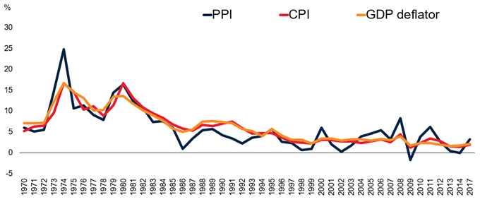
PPI vs CPI vs GDP Deflator

Source: World Bank

Sources of Inflation

Inflation can begin via many avenues in isolation or combination. Below are a few of the primary sources of inflation that can distress any nation across the globe:

Exchange Rates

A weakening local currency means that more local currency is required to purchase imports. This increased cost gets passed on to the end consumer which can contribute to inflation.

Essential Commodity Prices

Most manufacturers require inputs to produce a certain good. These often come in the form of commodities such as iron ore or oil. If these inputs increase in price due, then those costs can be passed on to consumers and the higher costs are a form of inflation.

Interest Rates

Lower interest rates theoretically lead to more spending by consumers, ultimately resulting in greater demand and cost of goods; which should lead to inflation, all factors held equal.

Government Debt

Increases in government debt may infer that there is a greater potential of a government default, which leads to higher yields on treasury securities to compensate potential investors for the higher risk. The effect this has on the public is that more tax revenue will be allocated to the higher interest payments on government debt obligations which reduces living standards. Businesses in turn increase the prices of goods and services to offset the lessened government expenditures, and this can lead to inflation.

The sources listed above generally fall into two broad categories of inflation which are:

  1. Demand-Pull Inflation – This type of inflation comes as a result of an increase in aggregate demand inclusive of households, governments, foreign buyers and businesses.
  2. Cost-Push Inflation – Supply is the driver of inflationary pressure for cost-push inflation. When supply falls due to higher production costs, the outcome is higher final prices for consumers.

Consequences of Inflation

Value of Money

The most obvious penalty of inflation from a consumer point of view is the higher cost of goods and services. This translates to a decrease in the value of money as individuals can now purchase fewer goods and services with the same amount of money prior to an inflationary rise.

Wealth Gaps

The inequitable distribution of inflationary pressure amongst individuals can lead to changes in wealth. For example, individuals with loans during periods of high inflation will benefit as the real value of their debt repayments will fall over time while others may not.

Inflation Volatility

Fluctuating or erratic inflation data complicates business operations as businesses do not know where to set prices, and this can have a negative effect on the economy as both businesses and consumers adjust to the higher rates of inflation. Long-term business deals will also incur higher costs as volatile inflation causes a higher risk premia on hedging costs, which can reduce foreign investor confidence.

Central banks use of Inflation Targeting

Inflation targeting is quite simple in theory as involves a central bank setting a specific inflation goal in percentage terms. This strategy is achieved by manipulating monetary policy. The goal of inflation targeting allows central banks along with the public to have more clarity in terms of future expectations. The reason behind inflation targeting is control with regards to price stability, and price stability can be attained by governing inflation.

Generally an inflation target of 1% – 2% is familiar as it allows governments and central banks some flexibility at this low base. As a rule of thumb, any deviation greater than 1% either side of the targeted figure is cause for concern and has generally lead to policy intervention.

How do Governments Control Inflation?

There are many ways governments go about controlling inflation which can have knock-on effects (positive and negative) to the economy depending on current economic conditions. The most common way is via contractionary monetary policy which is used by central banks to curb inflation by restricting liquidity. This is achieved via 3 main avenues:

1. Decrease Money Supply

Decreasing money supply simply gives consumers less money to spend overall and should help limit inflation. One way this can be realized is by increasing interest on sovereign bond payments which can attract more investors to buy bonds.

2. Reserve Constraints

Restricting the amount of money banks are allowed to keep can influence the amount of money being lent to consumers. That is, if banks are required to keep higher amounts of money as a legal threshold, then naturally banks will have less money to lend. This should decrease consumer spending and thus, inflation.

3. Raising Interest Rates

Higher interest rates which result in fewer individuals willing to borrow and therefore leads to a decrease in spending. There’s also a greater opportunity cost of investing capital into a business given the higher rates of return that could be had through capital markets.

Global Inflation and Key Relationships

Advanced vs Developing Economies
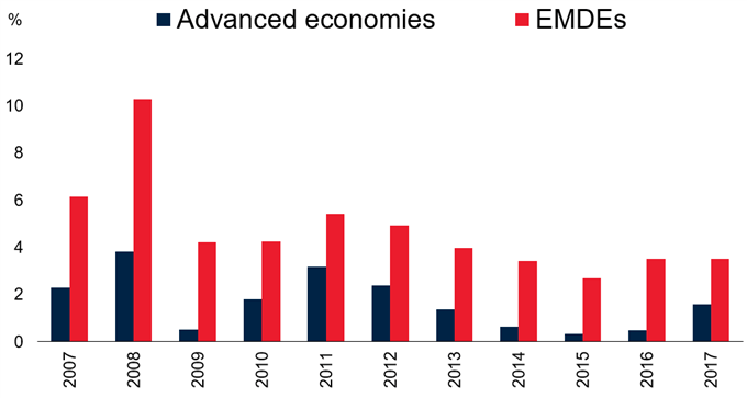
Advanced vs Developing economies

Source: World Bank

The chart above shows a consistent and logical pattern whereby the historical inflation rate in developed countries is generally less than emerging and developing economies (EMDE).There are two primary reasons behind this:

  1. EMDE generally have higher growth rates which can lead to excess demand.
  2. Volatile currencies are present in many EMDE which makes central banks’ management of monetary policy more difficult than those in advanced economies.

The Phillips Curve

The historical relationship between unemployment and inflation has been largely inverse which means that high levels of unemployment correlates with lower inflation and vice versa. The reason why the inverse relationship exists is best explained with basic economics. For example, an increase in aggregate demand which is a consequence of demand-pull inflation, results in higher prices of goods and services and lower unemployment. This lower unemployment means that there is more income available in the economy to spend on goods and services. Both elements have recurrent effects on one another and is best represented by the basic Phillips Curve (see chart below).
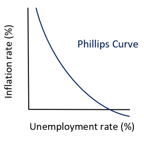
The Phillips Curve

Source: Created by Warren Venketas

Inflation: Conclusion

This article has demonstrated the wide reaching implication of inflation from more concentrated effects to wide-ranging systemic global impacts. Inflation is an important economic tool from a macroeconomic perspective but also can be powerful if understood and implemented within a trading strategy as inflation data can cause changes in price in many financial markets.

What is Forex Risk Management? Learn the Basics

What is Forex Risk Management? Learn the Basics

What is forex risk management?

Forex risk management comprises individual actions that allow traders to protect against the downside of a trade. More risk means higher chance of sizeable returns – but also a greater chance of significant losses. Therefore, being able to manage the levels of risk to minimize loss, while maximizing gains, is a key skill for any trader to have.

How does a trader do this? Risk management can include establishing the correct position size, setting stop losses, and controlling emotions when entering and exiting positions. Implemented well, these measures can prove to be the difference between profitable trading and losing it all.

Top 5 Fundamentals of Forex Risk Management

1. Appetite for Risk

Working out your appetite for risk is central to proper forex risk management. Traders should ask: How much am I willing to lose in a single trade? This is particularly important for the most volatile currency pairs , such as certain emerging market currencies . Also, liquidity in forex trading is a factor that affects risk management, as less liquid currency pairs may mean it is harder to enter and exit positions at the price you want.

If you don’t know how much you are comfortable with losing, your position size may end up too high, resulting in losses that may affect your ability to take on the next trade – or worse.

Let’s say 50% of your trades are winners. In the long term, mathematically you can expect to have runs of multiple losing trades in a row. Over a trading career of 10,000 trades, the odds suggest that you will face 13 sequential losses at some point. This underlines the importance of knowing your appetite for risk, as you need to be prepared, with sufficient money on your account, for when bad runs hit.

So how much should you risk? A good rule of thumb is to only risk between 1 and 3% of your account balance per trade. So, for example, if you have an account of $100,000, your risk amount would be $1,000-$3,000.

2. Position Size

Selecting the right position size , or the number of lots you take on a trade, is important as the right size will both protect your account and maximize opportunities. To select your position size, you need to work out your stop placement, determine your risk percentage and evaluate your pip cost and lot size. For more on how to do these things, click on the link above.

3. Stop Losses

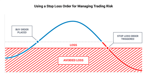
Using stop loss orders – which are placed to close a trade when a specific price is reached – is another key concept to understand for effective risk management in forex trading. Knowing the point in advance at which you want to exit a position means you can prevent potentially significant losses. But where is this point? Broadly, it’s whatever point your initial trading idea is invalidated. For more detail on this concept, click on the ‘Using stop loss orders’ link above.

How to use a stop loss order for managing trading risk

Traders should use stops and also limits to enforce a risk/reward ratio of 1:1 or higher. For 1:1, this means you are risking $1 to potentially make $1. Place a stop and a limit on each trade, ensuring that the limit is at least as far away from current market price as your stop.

The table shows how the outcomes of different risk-reward ratios can change a strategy:

Risk-Reward 1-1 1-2
Total Trades 10 10
Total Wins (40%) 4 4
Profit Target 100 pips 200 pips
Stop Loss 100 pips 100 pips
Pips Won 400 pips 800 pips
Pips Lost 600 pips 400 pips
Net Gain (-200 pips) 200 pips

As can be seen in the table, if the trader was only looking for one dollar in reward for every one dollar risked, the strategy would have lost 200 pips. But by adjusting this to a 1-to-2 risk-to-reward ratio, the trader tilts the odds back in their favor (even if only being right 40% of the time). For a full breakdown of this concept, read more on risk reward ratios for forex .

4. Leverage

Leverage in forex allows traders to gain more exposure than their trading account might otherwise allow, meaning higher potential to profit, but also higher risk. Leverage should, therefore, be managed carefully.

While researching how traders fared based on the amount of trading capital being used, DailyFX Senior Strategist Jeremy Wagner found that traders with smaller balances in their accounts, in general, carried much higher leverage than traders with larger balances. However, the traders using less leverage saw far better results than the smaller-balance traders using levels over 20-to-1. Larger-balance traders (using average leverage of 5-to-1) were profitable over 80% more often than smaller-balance traders (using average leverage of 26-to-1).

Based on this information, at least when starting out, it’s advisable for traders to be very wary of using leverage and to be mindful of the risks it poses.

5. Controlling Your Emotions

It’s important to be able to manage the emotions of trading when risking your money in any financial market. Letting excitement, greed, fear or boredom affect your decisions may expose you to undue risk. To help you take your emotions out of the equation and trade objectively, maintaining a forex trading journal or log can help you refine your strategies based on prior data – and not on your feelings.

What is the VIX? A Guide to the S&P 500 Volatility Index

What is the VIX? A Guide to the S&P 500 Volatility Index

What is the VIX in the stock market?

The VIX was created by the Chicago Board Options Exchange (CBOE) in 1990 to act as a benchmark for measuring expectations about future stock market volatility. It’s a real-time index which reflects market participants’ expectations of volatility over the next 30 days.

At the most basic level the VIX index is constructed using weekly and traditional SPX index options and their levels of implied volatility. One can think of implied volatility as expected volatility derived from market participants’ activity in the options market. Understanding why the VIX behaves inversely to the S&P 500 is important because the volatility index acts as a measure of market sentiment, hence the reason it is called a “fear barometer”.

What is the relationship between vix and S&P 500 (SPX)?

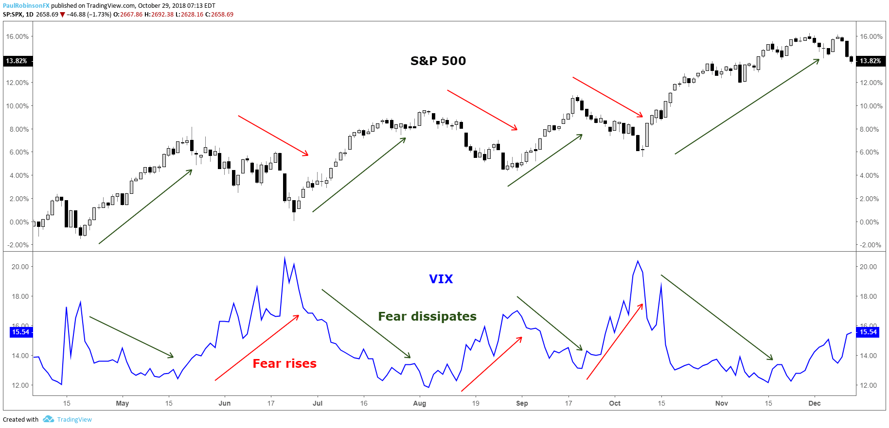
The S&P 500 VIX has a propensity to rise in bearish stock market environments and fall or remain steady during bullish environments. This happens because of the long-term bullish bias of the stock market and the fact that the VIX is calculated using implied volatility.

Implied volatility goes up when there is strong demand for options, and this typically happens during declines in the price of the S&P 500 as market participants (who are collectively bullish) are quick to buy protection (put options) for their portfolios.

When the S&P 500 rallies we see demand for protection dissipate and as a result a decline in the VIX. This process in recent years has become exasperated, in all likelihood, because the VIX has gone from just a market gauge of volatility to a tradable asset class through product offerings on various futures, equities, and options exchanges.

VIX rises when the S&P 500 falls

S&P 500 VIX correlation

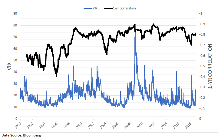
The S&P 500 VIX correlation is simply how the S&P 500 and the VIX move relative to one another. From the chart above it’s easy to see the strongly negative correlation between the stock market and the VIX. Stock market slumps lead to spikes in the index. Dating back the beginning of the VIX in 1990, the correlation between daily changes in the S&P 500 and VIX is -77%. Over the past 10 years the inverse correlation has become even stronger at -81%, while prior to October 2008 it was -74%.

The tighter relationship could very well be attributed to the various products introduced over the past 10-15 years which allow market participants to trade the VIX. As said earlier, this would also make sense as to why we are also seeing larger spikes in the VIX when the market weakens, as trading of the VIX itself is causing exaggerated moves in implied volatility.

The relationship between the S&P 500 and the VIX has largely been consistent and reliable over the years, though. The rolling 1-year correlation between daily changes has on average been around -83% over the past 10 years, staying within a relatively tight range of -70% to -90%.

S&P 500 VIX chart: One-year rolling correlation

VIX has a strong inverse correlation to the S&P 500 over the long-term

Using VIX to predict S&P 500 Volatility

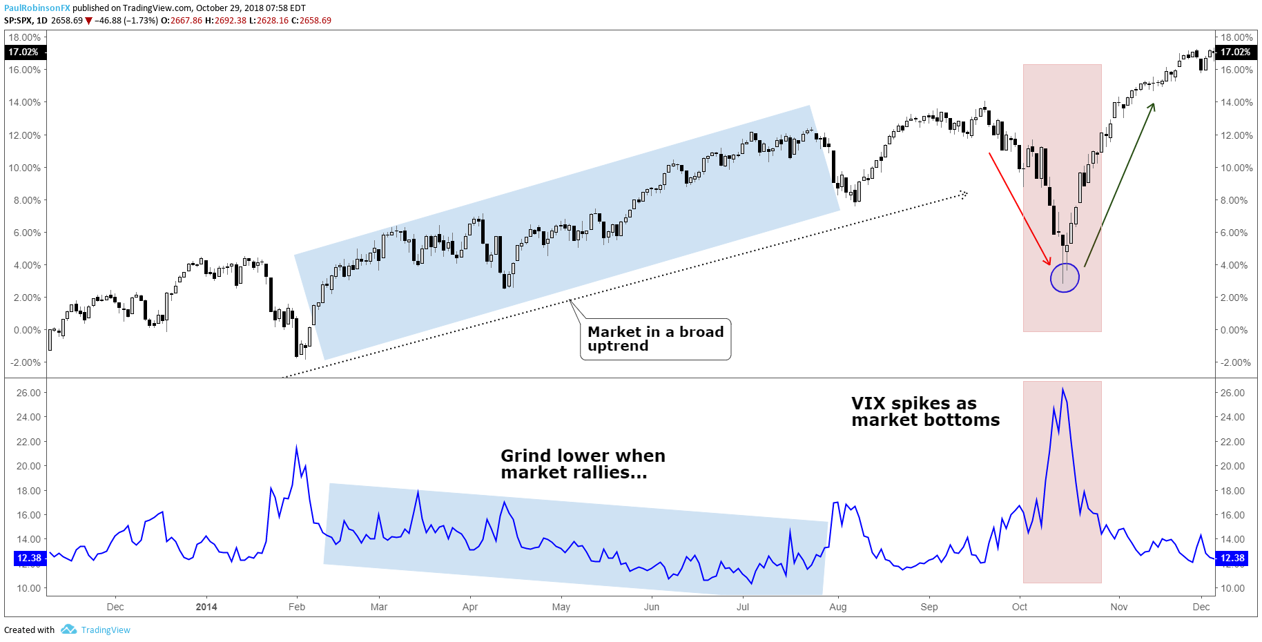
The S&P500 VIX can be used to identify market turns, more specifically bottoms. Because the stock market tends to rise in a gradual fashion the VIX too will decline in a gradual to sideways fashion. This can lead to very low levels which warn of complacency as investors feel no need for protection, but these periods can last long enough that using the VIX as a sell signal can be rendered largely ineffective.

However, because the S&P 500 is long-biased by nature, when there are declines investors buy protection (put options) quickly, driving up the VIX. Often there is an overreaction by market participants when the market declines, hence the reason why the VIX is called a “fear barometer”.

The spike-like behavior which the VIX exhibits during times of market stress can be a timely signal for determining when selling has become overdone and the market is due to bounce or even bottom for a longer-term move higher. This strategy is typically best employed when the VIX ‘signal’ arrives within the context of a generally bullish trend in the S&P 500.

S&P500 VIX chart: Spikes can be used to indicate trading bottoms

VIX moves lower to sideways in bullish markets, spikes during sell-offs

Circling back around to the complacency factor seen when the VIX is at very low levels, there is a nuance to this which can help identify when the stock market may be nearing a turning point to the downside, but they don’t happen frequently. When the VIX and S&P 500 both rise together over a period of time it can indicate growing instability in the trend which sets the market up for a sell-off.

Using S&P 500 volatility for risk management

When trading the S&P 500 there should be an inverse relationship between trading size and market volatility, or the VIX. One common mistake traders make is that they will simply trade a fixed lot size regardless of the distance their stop-loss is away from the entry price. This means the at-risk amount of capital will be highly variable (likely due to levels of volatility) and thus lead to inconsistent results. Additionally, a trader is putting themselves at greater risk when they should be doing the opposite.

A prudent approach to risk management is to determine how much of your capital you are willing to risk per trade and then adjust the trading size accordingly. For example, if you are willing to risk 1% on an S&P 500 trade and have a 10-point stop-loss, and have another trade where you are willing to risk 1%, but with a 5-point stop-loss, for both trades to equal 1% in risk the second trade would need to be twice as large as the first trade given the distance to the stop-loss. This provides a dynamic approach to position-sizing when trading the S&P 500 for more consistent results.

Average True Range (ATR) and the VIX

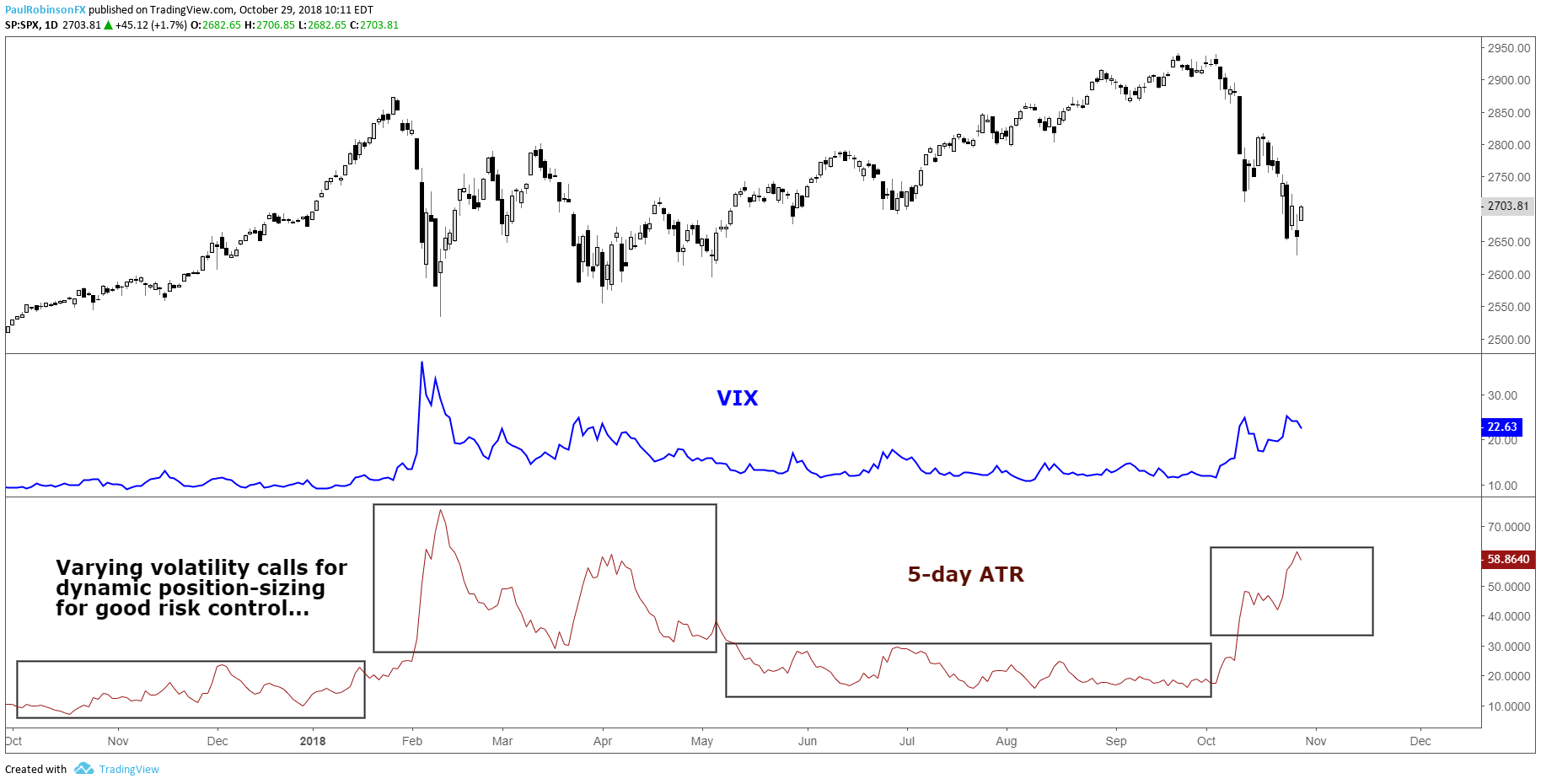
On average, the distance to your stop-loss will largely depend on the level of the VIX. Another way to measure volatility is with ATR (Average True Range). From the chart below, you can see that ATR and VIX look very similar, despite ATR using historical data and the VIX calculation relying on an options pricing model. When the VIX spiked so did the trading ranges of the S&P 500, which means a trader using a dynamic position-sizing strategy would adjust their trading size down to account for the new level of volatility. Simply put, if you are risking specific amounts of capital like in the example above, versus trading fixed lots, then you will be adjusting dynamically with S&P 500 volatility. For more on the topic of risk management, check out this article and video on sound risk management techniques.

S&P 500 VIX & ATR (Changing volatility requires changes to trading size)

As volatility changes (ATR/VIX) so should position sizes

S&P 500 and VIX Key takeaways

To summarize, understanding stock market volatility and the CBOE Volatility Index (VIX) is important for trading equity indices. There are benefits to understanding the nature of volatility from both an analytical and risk management standpoint. Like all things, getting a feel for the relationship between the VIX and the S&P 500 will take a little experience to get a handle on, but well worth the time.


Nasdaq Index, Dow Jones, S&P 500 News: Overall Earnings Exceed Expectations, Stocks Rally

Nasdaq Index, Dow Jones, S&P 500 News: Overall Earnings Exceed Expectations, Stocks Rally

Stock Futures Hold Steady

Stock futures remained relatively unchanged Friday morning, following the S&P 500’s historic surge to 5,000. This notable milestone was achieved during Thursday’s intraday trading. Dow Jones Industrial Average futures were static, while S&P 500 and Nasdaq 100 futures saw modest gains of 0.1% and 0.3%, respectively.

At 11:17 GMT, Dow futures are trading 38820.00, down 4.00 or -0.01%. S&P 500 Index futures are at 5021.50, up 3.75 or +0.07% and Nasdaq-100 Index futures are trading 17907.25, up 39.00 or +0.22%.

S&P 500’s Historic Climb

The S&P 500 briefly topped the 5,000 mark, reaching a peak of 5,000.40, before settling just below this threshold. This rise represents a significant journey since April 1, 2021, when the index first surpassed 4,000. Factors such as robust earnings, easing inflation, and a resilient economy have contributed to a 4.8% increase in the S&P 500 this year. Ryan Detrick of Carson Group highlights the psychological impact of crossing such significant numerical milestones.

Earnings Season Strength

The majority of S&P 500 companies reporting this quarter have exceeded expectations, with an 80.6% beat rate. This performance surpasses the typical 67% rate observed since 1994. However, Pinterest shares dropped 9% post-earnings, reflecting weaker-than-anticipated forecasts and revenues, despite a mitigating announcement of a Google app deal. Conversely, Cloudflare’s shares surged 18% following strong quarterly results and optimistic guidance.

Treasury Yields and Economic Data

U.S. Treasury yields were stable as investors considered recent economic data and the Federal Reserve’s interest rate trajectory. The 10-year Treasury yield held at 4.1715%, with the 2-year yield at 4.4651%. The market is digesting the latest jobless claims, which were slightly below expectations, suggesting continued labor market strength. This could influence the Fed’s interest rate decisions, with indications of fewer rate cuts than anticipated.

Anticipated Earnings and Data

Investors are now looking ahead to Pepsi’s earnings report, expected before Friday’s opening bell. Additionally, upcoming economic data, including January’s consumer price index, are keenly awaited.

Market Forecast

Given the resilience shown in earnings and economic indicators, the market outlook is bullish. The S&P 500’s ascent to 5,000, coupled with strong earnings reports, suggests underlying strength.

However, the steady Treasury yields and cautious Fed stance indicate a balanced approach in the short-term. Investors should monitor upcoming economic data, particularly inflation figures, for more directional cues.

Technical Analysis

Daily E-mini S&P 500 IndexThe E-mini S&P 500 Index is trading higher in the pre-market session, as investors try to build on its successful close over the psychological 5000 barrier.

This level is now minor support. The main support is a swing bottom at 4866.00. A trade through this level will change the main trend to down. This move would likely put the uptrending 50-day moving average at 4809.83 on the radar.

Despite the bullish momentum, there are some concerned about an overpriced market, given the widening distance between the current price at 5023.50 and the 50-day MA at 4809.83.

Trading the Gold-Silver Ratio: Strategies and Tips

Trading the Gold-Silver Ratio: Strategies and Tips

WHAT IS THE GOLD-SILVER RATIO?

The gold-silver ratio is simple. It is the number of silver ounces you would need to trade to receive one ounce of gold at current market prices. For example, when gold price is trading at $1000 per ounce and silver price is trading at $16.67 per ounce the gold-silver ratio will be equivalent to 60.

  • The gold to silver ratio has averaged around 60 from 2001 to 2017. With highs breaching 80 (ounces of silver to one ounce of gold) and lows sinking to around 40.
  • The ratio tends to increase during times of economic distress. The cause of this relationship is due to gold generally outperforming silver during recessions, leading to increases in the ratio.
  • The ratio peaked at 100 in 1991 when silver prices dropped to extreme lows.

HOW THE GOLD-SILVER RATIO WORKS

  • When the gold price increases faster than the silver price the ratio will increase .
  • When the silver price increases faster than the gold price the ratio will decrease .
  • When the gold price decreases faster than the silver price the ratio will decrease.
  • When the silver price decreases faster than the gold price the ratio will increase.

Source: Bloomberg data

The graph above shows the gold to silver ratio for the past several decades. In 1991 silver was trading at extremely low prices- causing a peak in the gold-silver ratio, denoted by the blue circle in the graph above.

It is also worth noting the spike in the ratio during the 2008 subprime-mortgage crisis, caused by surging gold prices and silver not performing as well. This is denoted by the red circle in the graph above.

HOW TO TRADE THE GOLD-SILVER RATIO

There are many ways to use the ratio to your advantage. Keep reading for the top two strategies on trading the gold-silver ratio.

1) USING THE GOLD-SILVER RATIO TO DETERMINE THE METAL WITH THE STRONGEST TREND AND TRADE IT:

Traders can use the gold-silver ratio to determine which metal may outperform the other and then place a trade accordingly.

A trader could use these five steps to enter a trade on either gold or silver using the ratio:

1) Determine the trend on a gold-silver ratio chart by adding trend lines to the chart. You can use DailyFX’s chart to view the gold-silver ratio by entering “XAUUSD/XAGUSD” in the search bar.

2) Using the time-frame of your choice, determine the trend on gold and silver individually.

3) Use this table to help you determine a bias:

GOLD-SILVER RATIO TREND GOLD AND SILVER TREND SIGNAL
Gold-Silver RatioUptrend Gold and silver inUptrend Buy Gold
Gold-Silver RatioUptrend Gold and Silver inDowntrend Sell Silver
Gold-Silver RatioDowntrend Gold and Silver inUptrend Buy Silver
Gold-Silver RatioDowntrend Gold and Silver inDowntrend Sell Gold

4) Identify trading opportunities using price action or technical indicators time entries in the direction of the trend.

5) Identify a trade size appropriate for the account size and set stop-losses and take-profits and execute the trade.

Here’s an example using the five steps:

1) Let’s say we open our gold to silver ratio chart on 8 February 2016.We draw our trend lines and the trend lines indicate that the ratio is in a current uptrend as shown in the chart below showing a four-hourly timeframe.

2) Our next step is to determine the individual trend for gold and silver. So, we open the charts and draw our trend lines and notice that both gold and silver are trending upwards as shown in the charts below.

3) The table above indicates that when the gold-silver ratio is trending upwards and gold and silver are both in an uptrend we should buy gold because it has been outperforming silver.

GOLD-SILVER RATIO UPTREND GOLD AND SILVER IN UPTREND BUY GOLD

4) Since the beginning of February, gold has increased drastically in price. We should wait for a modest pull-back before attempting to enter the market. Once we do enter the market, we can place our stop-loss below the trend line and our take-profit above the previous high to ensure a positive risk-reward ratio on the trade.

5) We determine an appropriate trade size for our account, execute the trade and set our stop-loss and take profit.

2) TRADING THE HIGHS AND LOWS OF THE GOLD-SILVER RATIO:

There may be times when the ratio reaches historic extremes. When it is near these points, a reversal of the ratio is at risk. For example, when the gold-silver ratio reaches for historical highs (from 80 to 100) the idea is that the price of gold is expensive relative to the price of silver. When the gold-silver ratio reaches for historical lows (from 60 to 40) gold is seen as cheaper relative to silver.

Because the metals are correlated though driven by different factors, they tend to be limited in their willingness to run beyond a gold-silver ratio north of 80-100 or below 60-40, and those tend to be at turning points because the ratio has picked up on a likely abrupt turning points in markets.

The chart below shows times when the ratio was at all-time highs- red circles and all-time lows-blue circles.

Traders can use the table below as a guide to trade the metals when the gold-silver ratio at risk for a reversal:

GOLD-SILVER RATIO EXTREME GOLD AND SILVER TREND TRADE SIGNAL
Gold-Silver RatioHistorical High Gold and Silver inUptrend Long Silver
Gold-Silver RatioHistorical High Gold and Silver inDowntrend Short Gold
Gold-Silver RatioHistorical Low Gold and Silver inDowntrend Short Silver
Gold-Silver RatioHistorical Low Gold and Silver inUptrend Long Gold

It is very seldom that the gold-silver ratio reaches for these historic highs and lows, but when it does, it could offer good opportunities. Still, it is important to manage your risk because the ratio has been known to breach these historical levels.

Gold, Silver Watching Seasonal CPI Adjustments on Friday

Gold, Silver Watching Seasonal CPI Adjustments on Friday

Gold Settles into Narrowing Pattern as Yields, USD Edge Higher

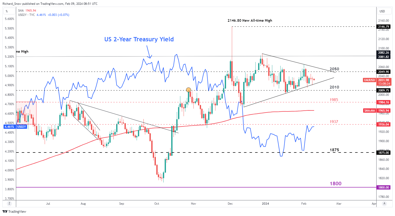
Gold entered into a narrowing pattern at the end of last year (with hindsight), seeing gold price rallies and selloffs relatively more contained. Prices rose at the end of 2023 but since then, have entered into more of a consolidatory phase, with prices broadly being contained between $2050 and $2010.

Intra-day price ranges reveal the market is active but closing prices over the last two sessions, and potentially today, witness flat closing prices. Yesterday’s test and rejection of trendline support sees gold stabilizing around opening levels, as the yellow metal is on track to end the week flat or little changed.

The safe haven demand for gold has waned as markets appear to have become desensitised to geopolitical tensions and conflicts currently ongoing. Gold has therefore, taken its cue from dollar and treasury markets. The blue line depicts the US 2-year Treasury yield which exhibits an inverse relationship with gold prices and the recent lift in yields may see a marginally lower close this week.

Gold (XAU/USD) Daily Chart

image1.png

Something to keep an eye on at 13:30 GMT today is the Bureau of Labor Statistics’ annual update of seasonal adjustment factors for past CPI prints. This affects the month-on-month (MoM) rise/fall in inflation and leaves year-on-year (YoY) measures unchanged. Higher MoM CPI revisions may see the dollar strengthen as rate cut bets continue to be pared back, while lower revisions could weigh on yields and the dollar as the disinflation trend would appear to be moving in the right direction.
Silver Prices on Track for a Flat Week

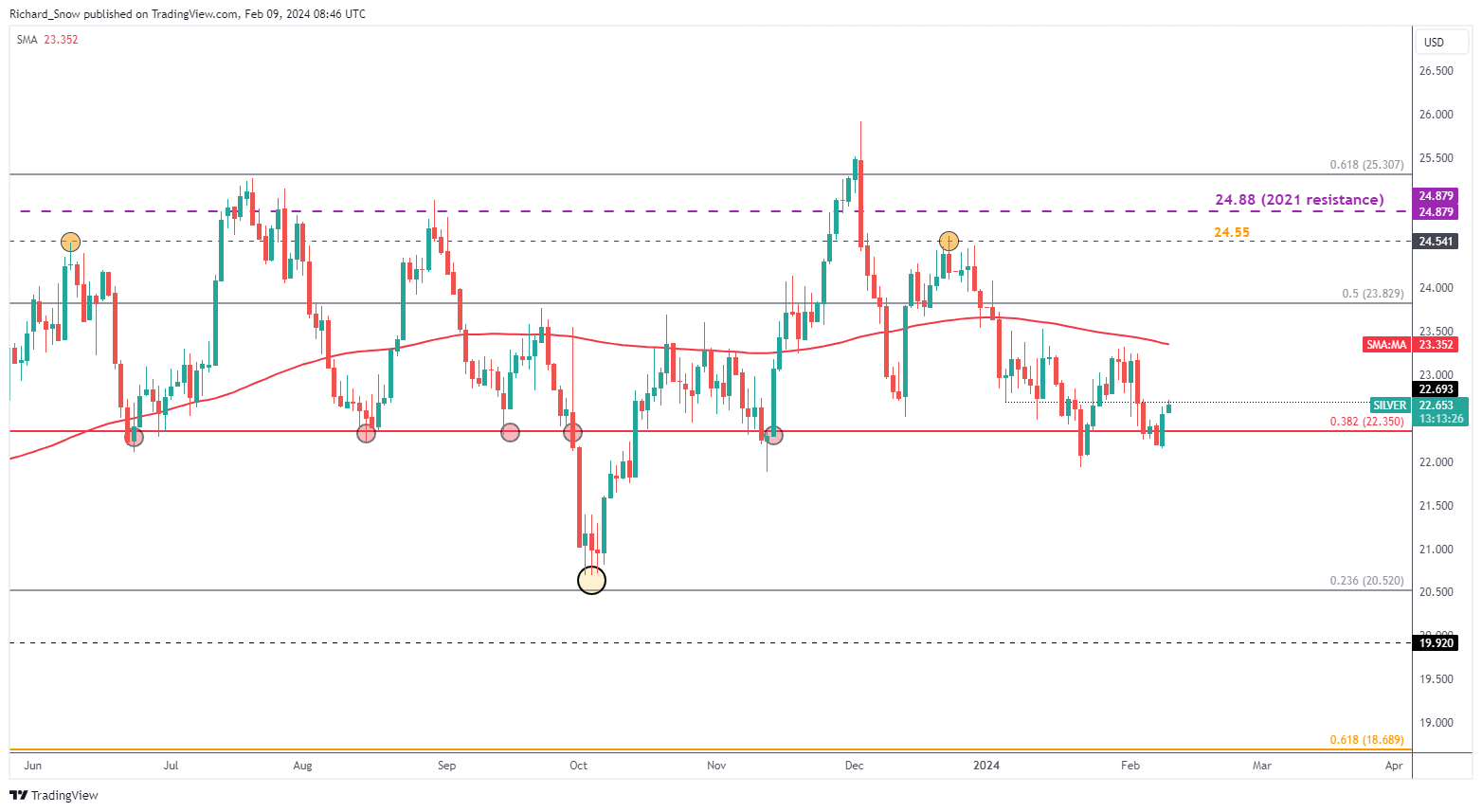
Silver sees a move higher into the end of the week, reclaiming lost ground off the back of last Friday’s NFP blowout. The move does appear unconvincing unless we see a close above $22.70 – the prior low right at the start of the year.

In addition, silver prices have shown little regard for the significant level of $22.35 which previously kept bears at bay, supporting prices and providing a pivot point on more than one occasion. The level pertains to the 38.2% Fibonacci retracement of the major 2021 to 2022 decline. The Fib level does present us with a potential support level in the short-term, with the swing low at $21.33 thereafter.

Silver (XAG/USD) Daily Chart

image2.png

EURUSD Ticks Lower As Weaker German Inflation Confirmed, ECB Still In A Bind

EURUSD Ticks Lower As Weaker German Inflation Confirmed, ECB Still In A Bind

The Euro was weaker but not far from its opening levels in European trade Friday, in a session with little to offer in the way of scheduled trading cues.
The big one on the EUR side of EUR/USD has already passed. Headline German inflation was confirmed at its weakest level for two and a half years. The Consumer Price Index rose by an annualized 2.9% in December, below November’s 3.1% and continuing the downtrend seen since the peaks above 8% in early 2023.

While inflation is heading in the right direction as far the European Central Bank is concerned, Germany presents a microcosm of European rate-setters’ problems. Prices may be weakening but they remain above target and vulnerable to resurgence thanks to any number of factors, from domestic wage bargaining to supply chain shocks thanks to conflict in Gaza and Ukraine.

And this comes against a backdrop of shaky economic growth. Global markets may be only too well aware that the Federal Reserve wants to wait until it has a clear inflation picture before cutting rates. The ECB’s position is if anything trickier. Growth is weaker, inflation stronger.

Still, for now markets seem content to believe that continued weak data will mean that record-high Eurozone rates will come down when next they move, and, although this may not happen soon, the prospect continues to keep the Euro in check.

It lost a lot of ground to the Dollar last week, when the Fed caused a huge pushing back of US rate-cut expectations, and hasn’t made much of it back.

However, as with other Dollar pairs, it is notable that recent trading ranges have been respected, which is likely to be the case at least until the monetary picture is more certain.

The ECB won’t set rates again until March 21, which is probably going to seem like an even longer time in the markets than it is. Central bankers’ comments will likely rule the market until then.

EUR/USD Technical Analysis

A graph of a stock market  Description automatically generated with medium confidence

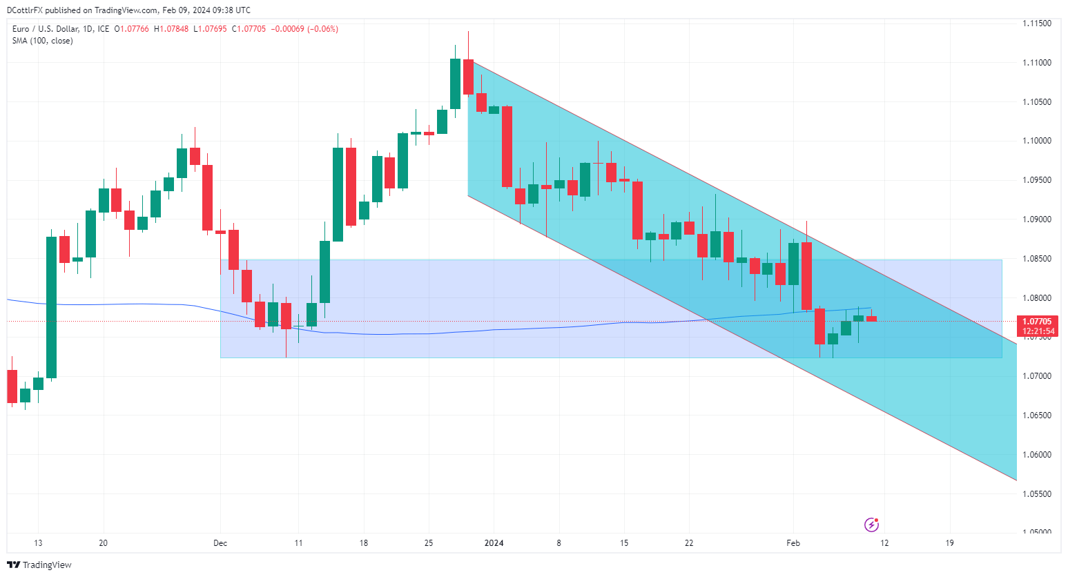
EUR/USD The Euro is bubbling away just below resistance at its 100-day moving average. The pair plunged below this during last week’s savage bout of US Dollar strength and hasn’t managed to retake it since. It comes in at 1.07868 which is where the bulls were beaten back on Thursday and where they’ve already retreated again early in Friday’s session.

While the broad downtrend from December remains in play the channel base hasn’t faced any serious test since early January. As such its validity as an indicator of substantial support may be fading out. However the trading band between December 5’s intraday high of 1.08594 and December 8’s low of 1.0752 would still seem to have some relevance as a possible directional indicator and , as it seems likely to face another downside test shortly, traders should keep an eye on it.

Breakout Ballistics in Trading and Analysis

Breakout Ballistics in Trading and Analysis

There’s but one problem with this scenario: Breakouts are unpredictable. So, for the trader that sees a range or a mean-reverting market to then approach that backdrop with breakout logic – they are, by default, expecting something new to happen that would change the paradigm that the trader’s analysis was built off of. So, generally speaking, breakouts are often approached as lower probability events.

But – this isn’t necessarily an entirely negative thing. When a breakout does take hold, the movement can be significant, which is one of the main allures of the market condition. So, if the trader can effectively manage the losses on the majority of trades that likely won’t continue to run after testing the breakout, there’s still the possibility of a profitable model even if the trader’s strategy is only seeing a success rate of 25 or 30%.

What is a Breakout

To put it simply, a breakout is a move to a fresh higher or low after a period of consolidation. Big picture, breakouts can exist on one minute charts the same as they can on daily or weekly charts. But, due to the ever-present noise of shorter time frames, traders are often focusing such approaches on chart time frames of an hour or longer for intra-day approaches or a day or longer for long-term approaches.

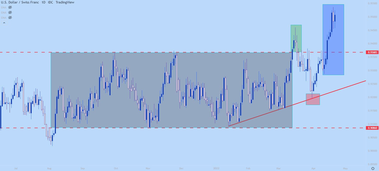
On the below daily chart of USD/CHF we’re looking at a range-bound formation in grey as both support and resistance held price action for an extended duration. This highlights equilibrium as both buyers and sellers are keeping prices fairly balanced here.

The initial breakout shows in green and that was the first breach of the formation which could be approached for breakout strategies.

Prices then pulled back into the prior range, finding support on the bullish trendline that was in-play before the break. This opened the door for trending strategies on the basis of the trendline hold (in red), after which buyers then posted another topside push with a fresh high following shortly after (in blue).

USD/CHF Daily Price Chart

How to Find Breakouts

Like both ranges and trends traders can choose to look for breakouts using either indicators or price action, with the latter approach being considerably more subjective. As such, many new traders will look to avoid that subjectivity by using an objective framework provided by the indicator.

One technical indicator that could be helpful in locating potential breakouts is the Average Directional Index, which gauges trend strength. Because the trader would be looking for a ‘new’ trend or theme, they would want to adopt a similar focus of range traders, looking for environments in which ADX was below a cut-off level such as 30, as we had looked at in our primer on the Average Directional Index (ADX) indicator.

On the below chart of USD/CHF, I’ve added the ADX indicator and notice how it remained below 30 for the entire duration of the range and the ensuing breakout.

USD/CHF Daily Price Chart

Breakouts Around News Events

One note of caution and a trap that many new traders will fall into is looking for breakouts around major news events. This is particularly relevant for Forex and futures markets, as equity markets will often attempt to release major drivers like earnings reports outside of market hours. But in the case of Forex pairs or for futures markets -announcements from Central Banks or data releases for inflation or employment numbers can create considerable intra-session volatility.

Read More on How to Trade Earnings Season

While these drivers can often compel breakouts, they can also be extremely messy with a lot of whipsaw, with resistance breaching temporarily before prices reverse after the data gets priced-in to the market. Trading around news events can be especially dangerous for new traders because liquidity is often lower (market makers are often risk averse around such scenarios) and that can lead to sharper moves in either direction.


Implied Volatility: What it is & Why Traders Should Care

Implied Volatility: What it is & Why Traders Should Care

WHAT IS IMPLIED VOLATILITY?

Implied volatility is a number displayed in percentage terms reflecting the level of uncertainty, or risk, perceived by traders. IV readings, which are derived from the Black-Scholes options pricing model, can indicate the degree of variation expected for a particular equity index, stock, commodity, or major currency pair over a stated period of time.

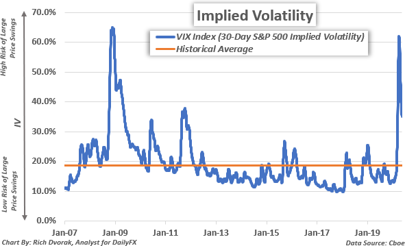
Implied Volatility Price Chart S&P 500-derived VIX Index

Implied volatility readings have a direct impact on the price of option contracts and are thus important metrics tracked by options traders. Several other market participants analyze and pay close attention to implied volatility as well seeing that useful insight that can be garnered and incorporated into a trading strategy. The well-known VIX Index, for instance, is simply the 30-day implied volatility reading derived from at-the-money S&P 500 option prices.

A high VIX level (i.e. percent), or implied volatility reading, indicates that stock market risk is relatively elevated and there is a greater chance of larger than normal price swings over the specified time frame. A greater range of potential outcomes, in turn, leads to higher implied volatility readings, and corresponds with a higher options contract price for the underlying asset.

This positive relationship between implied volatility and options contract price is true for both call options and put options. To be clear, this is assuming all other variables in the options contract pricing model are held constant. Aside from directly impacting option contract prices, there are multiple applications for analyzing implied volatility. Some examples include looking at differences between implied volatility and realized volatility, gauging market sentiment, identifying support and resistance levels, and finding relationships across asset classes.

IMPLIED VOLATILITY VS HISTORICAL VOLATILITY – WHAT IS THE DIFFERENCE?

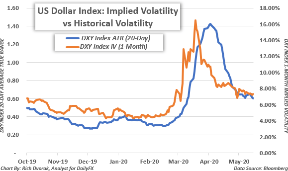
Implied volatility is the expected size of a future price change. Implied volatility broadly reflects how big or small of a move is anticipated to be over a particular time frame. On the other hand, historical volatility, or realized volatility, indicates the actual size of a previous price change. Historical volatility illustrates the overall level of market activity that has already been observed.

US Dollar Volatility Price Chart Realized vs Implied

The average true range (ATR) of an asset or security is an example of an indicator that illustrates historical volatility. Though implied volatility and historical volatility differ slightly in the regard of future expectations versus past observations, the two metrics are closely related and tend to move in similar patterns.

Implied volatility readings are typically higher when there is a large degree of uncertainty corresponding with potential for market impact – and often surrounds economic data releases or other scheduled risk events like central bank meetings. This can lead to larger price swings and thus can materialize into higher readings of realized volatility. Likewise, when historical volatility remains anchored during calm market conditions, or when perceived risk is relatively subdued, IV tends to be lower.

IMPLIED VOLATILITY CAN REFLECT MARKET RISK AND UNCERTAINTY

Implied volatility is a projection of how much market movement is anticipated – regardless of the direction. In other words, implied volatility reflects the expected range of potential outcomes and uncertainty around how high or low an underlying asset might rise or fall.

High implied volatility indicates there is a greater chance of large price swings expected by traders whereas low implied volatility signals that the market expects price movements to be relatively tame. Implied volatility measurements can also help traders gauge market sentiment considering IV broadly depicts the level of perceived uncertainty – or risk.

IMPLIED VOLATILITY TRADING RANGES CAN INDICATE TECHNICAL SUPPORT AND RESISTANCE LEVELS

Implied volatility measurements can be incorporated into various trading strategies as well. This is due to their usefulness for identifying potential areas of technical support and resistance. An implied volatility trading range is typically calculated under the assumption that prices will stay contained within a one-standard deviation move. Mathematically, this means that there is a 68% statistical probability that price action will fluctuate within the defined implied volatility trading range over a specified time frame.

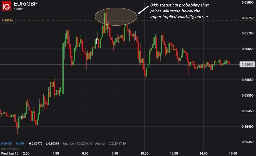
That said, if prices trade at the upper barrier of its pre-defined implied volatility trading range, then there is an 84% statistical probability that prices will gravitate lower and a 16% probability that prices will continue rising. On the other hand, if prices trade at the lower barrier of its pre-defined implied volatility trading range, then there is an 84% statistical probability that prices will drift higher and a 16% probability that prices will continue falling.

ADVANTAGES OF IMPLIED VOLATILITY AS A FOREX SIGNAL

Largely owed to the inherent mean-reverting characteristic of major currency pairs, implied volatility trading ranges typically serve as robust forex signals. For example, this EUR/GBP analysis that defined a 24-hour implied volatility trading range for EUR/GBP provided an illustrated example of how these technical barriers can help traders identify possible inflection points and trading opportunities.

EURGBP Price Chart Implied Volatility Trading Strategy Example

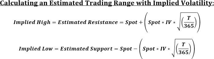
On 14 January 2020, spot EUR/GBP price action was trading at 0.8541 and its implied volatility measurement was clocked at 7.3% for the overnight (i.e. 1-day) options contract. Using these value inputs, and the options-derived trading range formula below, it was estimated that EUR/GBP would fluctuate between implied support of 0.8508 and implied resistance of 0.8574 over the next 24-hours with a 68% statistical probability.

Implied Volatility Chart Calculation of Trading Range Strategy

In other words, the calculated 24-hour trading range reflected a 1-standard deviation implied move of

+/- 0.0033 from spot, which meant that Euro-Pound volatility was expected to be contained within a 66- pip band around its then-current price of 0.8541 for the 15 January 2020 trading session.

As trading progressed and market activity unfolded, EUR/GBP jumped to an intraday high of 0.8578, but the currency pair closed the 15 January 2020 session at 0.8547 after spot prices pivoted sharply lower. This was driven by an influx of selling pressure that followed a rejection of its implied high technical barrier.

USING IMPLIED VOLATILITY TO TRADE COMMODITIES, STOCKS, & INDICIES

In addition to forex, implied volatility gauges can be incorporated into trading strategies for commodities, stocks, and indices. As mentioned above, measures of implied volatility can indicate the market’s overall level of uncertainty. Correspondingly, cross-asset implied volatility benchmarks tend to reflect useful relationships with their respective underlying markets and may provide insight as to where that market might head next.

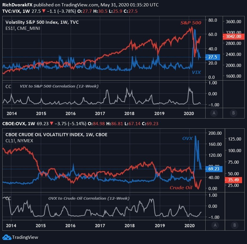
Implied Volatility Price Chart S&P 500 VIX and Crude Oil OVX

Arguably the most popular implied volatility benchmark is the S&P 500 VIX Index. The VIX Index typically rises amid turbulent market conditions and increasing uncertainty, though the ‘fear-gauge’ tends to soar during aggressive selloffs in stocks. In turn, the VIX generally holds a strong inverse relationship with the S&P 500.

The OVX Index, which reflects 30-day expected crude oil price volatility, provides an example of another commonly cited IV benchmark. Seeing that the price of crude oil and stocks react similarly to deteriorating risk appetite, it is unsurprising that sentiment-linked crude oil frequently maintains a negative correlation with both the VIX and OVX.

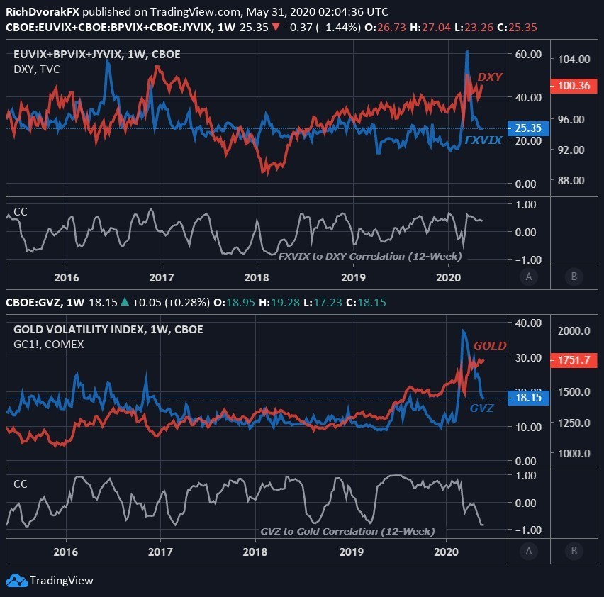
Implied Volatility Price Chart How to Trade Gold and US Dollar

Although this inverse relationship typically observed between an asset’s price and its implied volatility reading serves as a general rule of thumb, that is not always the case and there are certain exceptions. The correlation of price with implied volatility is dynamic, meaning it is constantly changing, which corresponds with a relative strengthening or weakening from their historical relationship.